Blog Entry Number One
To get my new website finally online, I want to add something to the blog section. Here in the future mostly stuff should be published that is related to archaeology and statistics using R.
To start I want to add a bit that helps to understand the relationship of several items within a collection of data. To be more specific, how can I explore the correlation of lets say pottery types or in this case animal species in the archaeological remains of different sites. Do specific combination occure regularily, so that it might be the case that they are functional related?
As an example I will use the animal remains from sites of the so called Funnelbeaker Culture, on which I recently published an article that is still under review. The data mostly originate from the collection in an article of Jan Steffens (2005), but there are some additions from an [unpublished (?) master thesis of Peter Imperiale] [@Imperiale2001]. You may like to download the data set.
Within this data set the question was/is, how the different animal species do correlate, and how this can be explored/visualised intuitively. The most obvious candidate was a network that display the interdependence of those species. When two species correlate positively and significant, their representation in the network should be linked by a connection.
To start this enterprise, we first load the data into our R environment:
animals <- read.csv2("tbk_animals.csv") #note that it is the "continental" csv version!

library(knitr)
kable(animals)| id | site | Hausrind | Hausschwein | Schaf.Ziege | Hund | Pferd | Rothirsch | Reh | Elch | Ur | Wildschwein | Braunbär | Dachs | Marder | Iltis | Fischotter | Wolf | Fuchs | Luchs | Wildkatze | Biber | Feldhase | Robbe | sonstige | summe |
|---|---|---|---|---|---|---|---|---|---|---|---|---|---|---|---|---|---|---|---|---|---|---|---|---|---|
| 1 | Alsleben | 46 | 1 | 8 | 0 | 0 | 2 | 0 | 0 | 2 | 1 | 0 | 0 | 0 | 0 | 0 | 0 | 0 | 0 | 0 | 0 | 0 | 0 | 0 | 60 |
| 2 | Basedow | 87 | 26 | 15 | 9 | 29 | 265 | 71 | 10 | 25 | 81 | 2 | 4 | 0 | 0 | 0 | 0 | 0 | 0 | 0 | 10 | 0 | 0 | 0 | 634 |
| 3 | Bebensee | 43 | 17 | 2 | 11 | 6 | 99 | 20 | 1 | 47 | 27 | 0 | 0 | 0 | 0 | 3 | 0 | 0 | 0 | 2 | 8 | 0 | 0 | 0 | 286 |
| 4 | Bistoft | 213 | 112 | 209 | 24 | 0 | 363 | 17 | 5 | 22 | 72 | 0 | 0 | 2 | 0 | 43 | 1 | 0 | 0 | 0 | 53 | 1 | 0 | 0 | 1137 |
| 5 | Dölauer Heide | 105 | 35 | 44 | 2 | 22 | 2 | 1 | 0 | 0 | 3 | 0 | 1 | 0 | 0 | 0 | 0 | 0 | 0 | 0 | 0 | 0 | 0 | 1 | 216 |
| 6 | Fuchsberg-Südensee | 624 | 94 | 44 | 18 | 5 | 45 | 15 | 0 | 20 | 46 | 0 | 0 | 0 | 0 | 0 | 0 | 0 | 0 | 1 | 3 | 0 | 0 | 7 | 922 |
| 7 | Glasow | 37 | 11 | 68 | 0 | 0 | 5 | 10 | 0 | 21 | 3 | 2 | 2 | 0 | 0 | 0 | 1 | 0 | 0 | 1 | 0 | 0 | 0 | 0 | 161 |
| 8 | Großobringen | 3064 | 0 | 570 | 161 | 129 | 248 | 28 | 1 | 0 | 0 | 14 | 1 | 0 | 0 | 0 | 0 | 2 | 1 | 0 | 5 | 0 | 0 | 0 | 4224 |
| 9 | Haldensleben | 45 | 5 | 6 | 0 | 0 | 0 | 0 | 0 | 0 | 0 | 0 | 0 | 0 | 0 | 0 | 0 | 0 | 0 | 0 | 1 | 0 | 0 | 0 | 57 |
| 10 | Heidmoor | 891 | 440 | 139 | 145 | 35 | 1707 | 336 | 162 | 93 | 515 | 6 | 35 | 17 | 6 | 46 | 35 | 1 | 1 | 46 | 579 | 1 | 29 | 17 | 5282 |
| 11 | Hüde I | 75 | 46 | 17 | 35 | 393 | 301 | 237 | 307 | 989 | 793 | 110 | 6 | 29 | 6 | 64 | 12 | 6 | 2 | 23 | 781 | 0 | 0 | 0 | 4232 |
| 12 | Neukirchen-Bostholm | 190 | 148 | 36 | 4 | 0 | 12 | 2 | 0 | 2 | 4 | 1 | 2 | 0 | 0 | 0 | 0 | 0 | 0 | 0 | 1 | 0 | 0 | 0 | 402 |
| 13 | Niedergörne | 60 | 29 | 39 | 0 | 0 | 6 | 1 | 0 | 0 | 0 | 0 | 0 | 0 | 0 | 0 | 0 | 0 | 0 | 0 | 0 | 0 | 0 | 0 | 135 |
| 14 | Runstedt | 67 | 7 | 0 | 0 | 2 | 0 | 0 | 0 | 0 | 0 | 0 | 0 | 0 | 0 | 0 | 0 | 0 | 0 | 0 | 0 | 7 | 0 | 0 | 83 |
| 15 | Schalkenburg | 1508 | 404 | 792 | 104 | 24 | 37 | 67 | 0 | 12 | 28 | 3 | 3 | 6 | 0 | 0 | 3 | 9 | 0 | 3 | 1 | 1 | 0 | 49 | 3054 |
| 16 | Siggeneben-Süd | 38 | 41 | 9 | 3 | 0 | 16 | 1 | 0 | 3 | 6 | 1 | 0 | 0 | 0 | 1 | 2 | 0 | 0 | 4 | 0 | 0 | 8 | 2 | 135 |
| 17 | Stinthorst | 15 | 18 | 6 | 2 | 8 | 151 | 31 | 13 | 5 | 30 | 5 | 1 | 1 | 0 | 0 | 0 | 1 | 0 | 0 | 3 | 0 | 0 | 0 | 290 |
| 18 | Süssau | 568 | 113 | 97 | 12 | 0 | 18 | 0 | 0 | 0 | 3 | 0 | 0 | 0 | 0 | 0 | 0 | 0 | 0 | 0 | 0 | 0 | 2 | 0 | 813 |
| 19 | Wangels FN | 164 | 8 | 57 | 11 | 1 | 65 | 23 | 0 | 13 | 11 | 1 | 0 | 1 | 0 | 1 | 0 | 0 | 0 | 0 | 0 | 0 | 5 | 9 | 370 |
| 20 | Wangels MN | 151 | 128 | 32 | 15 | 0 | 113 | 48 | 0 | 9 | 34 | 0 | 0 | 0 | 0 | 0 | 0 | 0 | 0 | 0 | 0 | 0 | 24 | 72 | 626 |
| 21 | Wolkenwehe | 2586 | 448 | 168 | 16 | 32 | 2875 | 416 | 16 | 104 | 288 | 0 | 8 | 1 | 0 | 8 | 2 | 8 | 0 | 8 | 456 | 0 | 8 | 0 | 7448 |
| 22 | Blandebjerg | 423 | 124 | 37 | 0 | 1 | 0 | 1 | 0 | 0 | 0 | 0 | 0 | 0 | 0 | 0 | 0 | 0 | 0 | 0 | 0 | 0 | 0 | 0 | 586 |
| 23 | Bundsø | 1405 | 1222 | 359 | 196 | 0 | 142 | 3 | 7 | 7 | 7 | 3 | 0 | 14 | 1 | 3 | 1 | 0 | 0 | 0 | 0 | 0 | 10 | 0 | 3380 |
| 24 | Fannerup | 183 | 106 | 149 | 10 | 7 | 46 | 10 | 0 | 13 | 16 | 0 | 1 | 0 | 0 | 3 | 0 | 1 | 0 | 0 | 0 | 0 | 17 | 0 | 562 |
| 25 | Lidsø | 672 | 66 | 137 | 49 | 0 | 0 | 2 | 0 | 0 | 0 | 0 | 0 | 0 | 0 | 0 | 0 | 0 | 0 | 0 | 0 | 0 | 11 | 1 | 938 |
| 26 | Lindø | 1293 | 659 | 421 | 30 | 1 | 90 | 0 | 0 | 0 | 5 | 3 | 0 | 0 | 0 | 3 | 1 | 0 | 0 | 0 | 0 | 1 | 0 | 1 | 2508 |
| 27 | Lyø | 297 | 85 | 59 | 0 | 0 | 8 | 0 | 0 | 0 | 0 | 0 | 0 | 0 | 0 | 0 | 0 | 0 | 0 | 0 | 0 | 0 | 25 | 0 | 474 |
| 28 | Sølanger | 15 | 1 | 29 | 34 | 0 | 60 | 128 | 0 | 0 | 96 | 0 | 0 | 0 | 0 | 8 | 0 | 9 | 0 | 3 | 0 | 1 | 16 | 1 | 401 |
| 29 | Spodsbjerg | 1978 | 891 | 588 | 101 | 4 | 179 | 8 | 0 | 0 | 8 | 1 | 0 | 0 | 0 | 4 | 1 | 4 | 0 | 0 | 1 | 0 | 23 | 101 | 3892 |
| 30 | Svaleklint | 35 | 0 | 0 | 0 | 0 | 126 | 65 | 0 | 0 | 0 | 0 | 0 | 0 | 0 | 0 | 0 | 0 | 0 | 1 | 5 | 0 | 10 | 0 | 242 |
| 31 | Troldebjerg | 10459 | 11632 | 2721 | 25 | 75 | 25 | 25 | 0 | 1 | 5 | 0 | 0 | 0 | 0 | 5 | 0 | 5 | 0 | 1 | 1 | 0 | 5 | 0 | 24985 |
| 32 | Löddesborg | 7 | 0 | 0 | 3 | 0 | 65 | 30 | 0 | 0 | 0 | 0 | 0 | 0 | 0 | 1 | 1 | 0 | 0 | 0 | 2 | 0 | 33 | 22 | 164 |
| 33 | Nymölla III | 7 | 0 | 0 | 0 | 0 | 74 | 23 | 0 | 0 | 0 | 1 | 0 | 0 | 0 | 8 | 0 | 3 | 0 | 2 | 0 | 0 | 21 | 6 | 145 |
| 34 | Brachnowko | 24 | 76 | 107 | 0 | 0 | 0 | 0 | 0 | 0 | 0 | 0 | 8 | 0 | 1 | 0 | 0 | 80 | 0 | 0 | 0 | 0 | 0 | 0 | 296 |
| 35 | Cmielow | 1579 | 566 | 276 | 112 | 57 | 36 | 44 | 3 | 0 | 44 | 3 | 5 | 0 | 0 | 0 | 3 | 3 | 0 | 0 | 5 | 0 | 0 | 0 | 2736 |
| 36 | Grodek | 1265 | 453 | 252 | 41 | 15 | 19 | 11 | 6 | 0 | 60 | 2 | 1 | 0 | 0 | 1 | 0 | 2 | 0 | 0 | 0 | 6 | 0 | 0 | 2134 |
| 37 | Kamin Lukawski | 1675 | 581 | 402 | 66 | 9 | 26 | 28 | 3 | 11 | 11 | 3 | 3 | 0 | 0 | 0 | 0 | 0 | 1 | 0 | 23 | 3 | 0 | 0 | 2845 |
| 38 | Kruska Podlotowa | 237 | 0 | 1 | 7 | 25 | 8 | 0 | 0 | 0 | 0 | 0 | 0 | 0 | 0 | 1 | 0 | 0 | 0 | 0 | 0 | 0 | 0 | 0 | 279 |
| 39 | Ksiaznice Wielkie | 150 | 137 | 25 | 31 | 0 | 9 | 26 | 0 | 0 | 5 | 0 | 0 | 0 | 0 | 0 | 1 | 0 | 0 | 50 | 0 | 2 | 0 | 0 | 436 |
| 40 | Mrowino | 359 | 78 | 93 | 8 | 3 | 29 | 3 | 0 | 0 | 12 | 7 | 0 | 0 | 0 | 0 | 0 | 0 | 2 | 0 | 1 | 0 | 0 | 0 | 595 |
| 41 | Pikutkowo | 103 | 26 | 14 | 69 | 3 | 1 | 0 | 0 | 0 | 0 | 1 | 0 | 0 | 0 | 0 | 0 | 0 | 0 | 0 | 0 | 0 | 0 | 0 | 217 |
| 42 | Podgaj | 197 | 19 | 94 | 0 | 0 | 2 | 0 | 0 | 0 | 0 | 0 | 0 | 0 | 0 | 0 | 0 | 0 | 0 | 0 | 0 | 0 | 0 | 0 | 312 |
| 43 | Srem | 1040 | 216 | 50 | 17 | 11 | 1 | 1 | 0 | 0 | 4 | 0 | 0 | 0 | 0 | 0 | 0 | 0 | 0 | 0 | 0 | 3 | 0 | 0 | 1343 |
| 44 | Strachow | 215 | 76 | 119 | 4 | 0 | 0 | 0 | 0 | 15 | 0 | 0 | 0 | 0 | 0 | 0 | 0 | 0 | 0 | 0 | 0 | 22 | 0 | 0 | 451 |
| 45 | Stryczowice | 327 | 36 | 48 | 71 | 0 | 0 | 0 | 0 | 8 | 4 | 0 | 0 | 0 | 0 | 0 | 0 | 0 | 0 | 0 | 0 | 3 | 0 | 5 | 502 |
| 46 | Szlachcin | 56 | 14 | 11 | 4 | 43 | 30 | 45 | 0 | 0 | 0 | 1 | 0 | 0 | 0 | 0 | 0 | 1 | 0 | 0 | 7 | 0 | 0 | 0 | 212 |
| 47 | Ustowo | 483 | 267 | 76 | 37 | 46 | 191 | 59 | 0 | 60 | 16 | 4 | 0 | 0 | 0 | 0 | 1 | 1 | 0 | 1 | 114 | 0 | 1 | 0 | 1357 |
| 48 | Zawichost-Podgorze | 1017 | 323 | 214 | 93 | 40 | 10 | 10 | 0 | 0 | 9 | 2 | 3 | 0 | 0 | 0 | 0 | 0 | 2 | 0 | 3 | 2 | 0 | 0 | 1728 |
| 49 | Makotrasy | 1636 | 373 | 173 | 50 | 14 | 31 | 1 | 0 | 5 | 10 | 2 | 0 | 0 | 0 | 0 | 2 | 0 | 0 | 0 | 2 | 7 | 0 | 2 | 2308 |
| 50 | Muldbjerg I | 33 | 0 | 3 | 0 | 0 | 665 | 116 | 0 | 0 | 5 | 0 | 0 | 2 | 0 | 115 | 0 | 0 | 0 | 0 | 179 | 0 | 0 | 4 | 1122 |
| 51 | Björnsholm | 1 | 0 | 2 | 0 | 0 | 6 | 9 | 0 | 0 | 3 | 0 | 0 | 1 | 0 | 0 | 0 | 2 | 0 | 0 | 0 | 0 | 0 | 0 | 24 |
| 52 | Saxtorp | 246 | 78 | 90 | 1 | 3 | 4 | 5 | 0 | 0 | 0 | 0 | 0 | 0 | 0 | 0 | 0 | 0 | 0 | 0 | 0 | 0 | 1 | 1 | 429 |
| 53 | Almhov - CT1 | 157 | 170 | 51 | 0 | 0 | 71 | 2 | 0 | 0 | 0 | 0 | 0 | 0 | 0 | 0 | 0 | 0 | 0 | 0 | 1 | 0 | 0 | 0 | 452 |
| 54 | Hunneberget | 85 | 50 | 36 | 16 | 0 | 19 | 27 | 0 | 0 | 0 | 0 | 0 | 1 | 0 | 0 | 0 | 1 | 0 | 1 | 3 | 0 | 7 | 2 | 248 |
| 55 | S.Sallerup 15H | 371 | 52 | 43 | 2 | 4 | 22 | 1 | 0 | 0 | 0 | 0 | 0 | 0 | 0 | 0 | 0 | 0 | 0 | 0 | 0 | 0 | 0 | 0 | 495 |
| 56 | Elinelund 2B | 314 | 59 | 14 | 2 | 0 | 1 | 0 | 0 | 0 | 0 | 0 | 0 | 0 | 0 | 1 | 0 | 0 | 0 | 1 | 0 | 0 | 0 | 1 | 393 |
| 57 | Hyllie station | 39 | 41 | 7 | 0 | 0 | 2 | 0 | 0 | 0 | 0 | 0 | 0 | 0 | 0 | 0 | 0 | 0 | 0 | 0 | 0 | 0 | 0 | 0 | 89 |
| 58 | Hyllie vattentorn | 40 | 27 | 0 | 1 | 0 | 0 | 0 | 0 | 0 | 0 | 0 | 0 | 0 | 0 | 0 | 0 | 0 | 0 | 0 | 0 | 0 | 0 | 0 | 68 |
| 59 | Hotelltomten | 79 | 68 | 7 | 0 | 0 | 2 | 0 | 0 | 0 | 0 | 0 | 0 | 0 | 0 | 0 | 0 | 0 | 0 | 0 | 0 | 0 | 0 | 0 | 156 |
| 60 | Skumparerget | 397 | 68 | 20 | 0 | 0 | 0 | 0 | 0 | 0 | 0 | 0 | 0 | 1 | 0 | 0 | 0 | 0 | 0 | 1 | 0 | 0 | 1 | 4 | 492 |
| 61 | Anneberg | 54 | 46 | 4 | 11 | 0 | 0 | 0 | 2 | 0 | 0 | 0 | 1 | 17 | 0 | 17 | 0 | 3 | 0 | 2 | 6 | 0 | 674 | 24 | 861 |
Displayed are now our sites with the NISP data of the species. For the construction of the network we now need a matrix, consisting of a row and a column for each species, filled with 1 for each situation when there is a positive significant correlation between the occurence of these both species. To archive this I used a modified snippet from the web (originally from Aleksandar Blagotić, function corstar.R), and the function corr.test from the library psych. I constructed this little function:
cornet <- function(x, y = NULL, use = "pairwise", method = "pearson", round = 3, row.labels, col.labels, ...) {

  require(psych)

  ct <- corr.test(x, y, use, method,adjust="bonferroni")    # calculate correlation
  r <- ct$r                             # get correlation coefs
  p <- ct$p                             # get p-values

  sig <- ifelse(p < .05, 1,0) # generate significance stars
  poscorr<-ifelse(r > 0, 1,0)

  m <- matrix(NA, nrow = nrow(r) , ncol = ncol(r)) # create empty matrix

  rlab <- if(missing(row.labels)) rownames(r) else row.labels # add row labels
  clab <- if(missing(col.labels)) {
    if(is.null(colnames(r)))
      deparse(substitute(y))
    else
      colnames(r)
  } else {
    col.labels # add column labels
  }

  rows <- 1:nrow(m)                     # row indices
  cols <- 1:ncol(m)                     # column indices

  m[rows, cols] <- sig*poscorr

  colnames(m) <- c( clab)           # add colnames
  rownames(m) <- c( rlab)           # add colnames
  m                                     # return matrix
}
With this at hand we can now prepare our data for the network plot:
adj <- cornet(na.omit(animals[,3:25]))## Lade nötiges Paket: psych## Warning in abbreviate(colnames(r), minlength = 5): abbreviate mit
## nicht-ASCII Zeichen genutztSecond thing we need for a nice plot is the function ggnet2 from the library GGally. This library has some dependencies, especially regarding ggplot and sna, so you might have to install them first!
library(GGally)But then:
ggnet2(adj, mode = "fruchtermanreingold", size = 24, label = rownames(adj), label.size = 3, alpha=0.8)## Lade nötiges Paket: network## network: Classes for Relational Data
## Version 1.13.0 created on 2015-08-31.
## copyright (c) 2005, Carter T. Butts, University of California-Irvine
## Mark S. Handcock, University of California -- Los Angeles
## David R. Hunter, Penn State University
## Martina Morris, University of Washington
## Skye Bender-deMoll, University of Washington
## For citation information, type citation("network").
## Type help("network-package") to get started.## Lade nötiges Paket: sna## sna: Tools for Social Network Analysis
## Version 2.3-2 created on 2014-01-13.
## copyright (c) 2005, Carter T. Butts, University of California-Irvine
## For citation information, type citation("sna").
## Type help(package="sna") to get started.##
## Attache Paket: 'sna'## Das folgende Objekt ist maskiert 'package:network':
##
## %c%## Lade nötiges Paket: scales##
## Attache Paket: 'scales'## Die folgenden Objekte sind maskiert von 'package:psych':
##
## alpha, rescale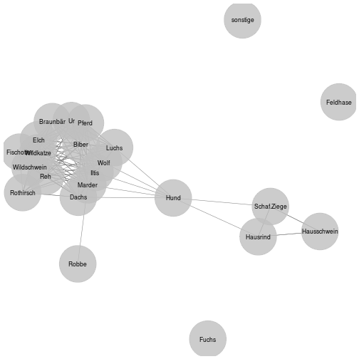
Voila! domestic species form one subnet (pig, cattle, sheep/goat), while most wild species form another subnet. There seem to be two separate spheres of interaction with the animals, indicating that there are two types of sites resp. activities: one is hunting, the other husbandry.